Constrained optimization

Exercise 1

Consider the problem:

$$\min_{\mathbf{x}\in\mathbb{R}^2}{J(\mathbf{x})=2x_1+x_2}\,\,\,\text{s.t.}\,\,\,x_1^2+x_2^2-2=0,$$

find all the extreme points, and
check the KKT conditions at the extreme points.

Exercise 2

Consider the half-space defined by (this is the exercise on page 353 n. 12.14 in the textbook):

$$H=\{\mathbf{x}\in\,\mathbb{R}^n\,\text{s.t.}\,\mathbf{a}^T\mathbf{x}+\alpha\geq 0\},$$

where $\mathbf{a}\in\,\mathbb{R}^n,\,\alpha\in\,\mathbb{R}$ are given:

formulate and solve the optimization problem of finding the point $\mathbf{x}^*\in H$ with the smallest Euclidean norm.

What is the Euclidean norm?

def: given $\mathbf{x}=(x_1,x_2,\ldots,x_n)\in\,\mathbb{R}^n$, the Euclidean norm of $\mathbf{x}$, denoted $\lVert \mathbf{x} \rVert$, is defined $\lVert \mathbf{x} \rVert=\sqrt{\sum^n_{i=1}{x_i^2}}$.

Euclidean distance — a. the norm in 2D ($\mathbb{R}^2$)

But what does it mean physically? Let's use the vector $\mathbf{x}$ as a Euclidean vector, that basically means a point in the Euclidean space $\mathbb{R}^n$. The Euclidean norm just measures the length of the vector $\mathbf{x}$ from the origin, as a consequence of the Pythagorean theorem.

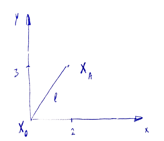
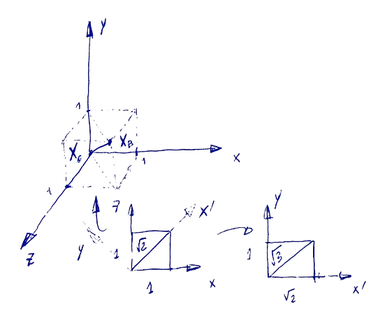
In the image (a) you can see what happens if you have a point $\mathbf{x}_A=(2,3)$. The norm is clearly $\lVert \mathbf{x}_A \rVert=\sqrt{13}$. This was easy; with the same principle, you can evaluate the norm in a more complex scenario, in any dimensional space. In 3D, constraint $y$-axis to zero first, and you will find the norm $\lVert \mathbf{x}_B' \rVert=\sqrt{2}$. Now put a "rectangle" with sizes $1\times \sqrt{2}$ as illustrated in (b) on the line that measures the norm that you have just found. You can see that the 3D norm is $\lVert \mathbf{x}_B \rVert=\sqrt{3}$ for the point $\mathbf{x}_B=(1,1,1)$.

The optimization problem can be written:

$$\min_{\mathbf{x}\in\mathbb{R}^n}{J(\mathbf{x})=\lVert\mathbf{x}\rVert^2} \,\,\,\text{s.t.}\,\,\,c_1(\mathbf{x})=\,\mathbf{a}^T\mathbf{x}+\alpha\geq 0,$$

where $c_1$ is an inequality constraint.

To find the point with the smallest Euclidean norm, we need to solve the optimization problem with Karush-Kuhn-Tucker (KKT) conditions.

What are the KKT conditions?

KKT condition is the first-order necessary condition for optimality (to be consistent conditions as it is a set of them), and you express them with the following th: suppose $x^*$ is a local minimum, $J,c_i$ are continuously differentiable. $\exists$ a Lagrange multiplier vector $\mathbf{\lambda}^*$ with components $\lambda_i^*, i\in\mathcal{E}\cup\mathcal{I}$ (meaning there is one $\lambda$ for each equality and inequality constraint) s.t.:

$\nabla_x\mathcal{L}(x^*,\lambda^*)=0$, this is the stationarity condition,
$c_i(x^*)=0,\,\forall i\in\mathcal{E}$, recall $\mathcal{E}$ are the equality constraints,
$c_i(x^*)\geq 0,\,\forall i\in\mathcal{I}$, recall $\mathcal{I}$ are the inequality constraints. Both this and the above one are primal feasibility conditions,
$\lambda_i^*\geq 0,\,\forall i\in\mathcal{I}$, this is the dual feasibility condition, and
$\lambda_i^*c_i(x^*)\geq 0,\,\forall i\in\mathcal{E}\cup\mathcal{I}$, this is the complementarity condition.

Ok. But what is the $\mathcal{L}$ Lagrange function or Lagrangian?

def: the Lagrangian is defined $\mathcal{L}(\mathbf{x},\mathbf{\lambda})=J(\mathbf{x})-\sum_{i\in\mathcal{E}\cup\mathcal{I}}{\lambda_ic_i(x)}$ where $\lambda_i$ are the Lagrange multipliers.

Lagrangian is named after Joseph-Louis Lagrange (1736-1823), other than a very interesting natural scientist (read some more about him), he reformulated Newton's mechanics into, well, Lagrange mechanics. Which is very important in the state-space representation of system evolution. That we use a lot in robotics!

In our case, the Lagrangian is:

$$ \mathcal{L}(\mathbf{x},\mathbf{\lambda})=\lVert\mathbf{x}\rVert^2-\lambda_1(\mathbf{a}^T\mathbf{x}+\alpha), $$

now, for simplicity let's suppose we are dealing with just one element in the vector $\mathbf{x}=x$ (and thus also $\mathbf{a}=a$). The first derivative of the Lagrangian is: $\nabla_x\mathcal{L}(x,\lambda)=2x-\lambda_1a$, and the second is: $\nabla_{xx}\mathcal{L}(x,\lambda)=2$.

We can notice that the second-order sufficient condition (we will see in detail in a latter exercise) is satisfied at all points ($2>0$). Let's use the KKT conditions to find the points with smallest Euclidean norm. The condition (1) can be also written:

$$ \nabla_x\mathcal{L}(x^*,\lambda^*)=2x^*-\lambda_1^*a=0,$$$$ x^*=\frac{\lambda_1^*}{2}a, $$

while the condition (5) implies that $\lambda_1$ or $c_1$ is zero:

$$ \lambda_1^*=0,$$$$ ax^*+\alpha=\frac{\lambda_1^* a^2}{2}+\alpha=0, $$

note that we wrote the above equation by substituting the value of $x^*$ that we found using the KKT condition (1). Depending on $\alpha$, there are thus two cases to satisfy KKT:

when $\alpha=0$, to have $ax^*=\frac{\lambda_1^* a^2}{2}=0$ we clearly need $x^*=0,\lambda_1^*=0$ [i], and
when $\alpha\neq 0$:
$ax^*+\alpha=0,\,ax^*=-\alpha\,\implies x^*=-\frac{\alpha}{a}$

$\lambda_1^*a^2\cdot\frac{1}{2}+\alpha=0\,\implies \lambda_1^*=-\alpha\frac{2}{a^2}$ [i].

Exercise 3

Consider the problem:

$$\min_{\mathbf{x}\in\mathbb{R}^2}{J(\mathbf{x})=x_1+x_2}\,\,\,\text{s.t.}\,\,\,x_1^2+x_2^2-1=0,$$

solve the problem by eliminating the variable $x_2$, and
show that the choice of sign is critical.

Exercise 4

Consider the problem of finding the point on the parabola $y=\frac{1}{5}(x-1)^2$ that is closest to $(1,2)$ in the Euclidean norm sense (this is the exercise on page 354 n. 12.18 in the textbook). We can formulate this problem as:

$$\min_{x,y\in\mathbb{R}}{J(x,y)=(x-1)^2+(y-2)^2}\,\text{s.t.}\,(x-1)^2-5y=0,$$

find all the KKT points and investigate if LICQ is satisfied,
which of these points are the solution, and
by substituting the constraint into $J$ (eliminating $x$) we get an unconstrained optimization problem. Show how the solution differs from the constrained problem.

The Lagrangian $\mathcal{L}(\mathbf{x},\mathbf{\lambda})=\mathcal{L}(x,y,\lambda_1)$ of the problem is:

$$\mathcal{L}(x,y,\lambda_1)=(x-1)^2+(y-2)^2-\lambda_1\left((x-1)^2-5y\right)$$ $$=(1-\lambda_1)(x-1)^2+(y-2)^2+5\lambda_1y,$$ $$\nabla_\mathbf{x}\mathcal{L}(x,y,\lambda_1)=\begin{pmatrix} \,\,\frac{\partial}{\partial x}\mathcal{L}(x,y,\lambda_1)\,\, \\ \frac{\partial}{\partial y}\mathcal{L}(x,y,\lambda_1) \end{pmatrix}=\begin{pmatrix} \,\,2(1-\lambda_1)(x-1)\,\, \\ 2(y-2)+5\lambda_1 \end{pmatrix},$$

Using the KKT condition (1) first, and (2) later, we have:

$$\nabla_\mathbf{x}\mathcal{L}(x^*,y^*,\lambda_1^*)=0\implies\begin{cases} 2(1-\lambda_1^*)(x^*-1)=0\\ \,\,\,\,\,2(y^*-2)+5\lambda_1^*=0 \end{cases}$$ $$\,\,\,\,\,\,\,\,\,\,\,\,\,\,\,c_1(x^*)=0\implies (x^*-1)^2-5y^*=0.$$

By solving these three equations, we obtain the following optimal points and the lambda multiplier: $x^*=1, y^*=0, \lambda_1^*=\frac{4}{5}$ [i]. Note that we have used just the KKT conditions (1—2); why? Well, think about it. So we have just an equality constraint here, which indicates that $c_1$ at the optimal point should be zero. Thus condition (5) is true as it contains $c_1$, which we say should be zero. Conditions (3—4) are both for inequality constraints only, so we don't consider them here.

What is LICQ?

The linear independence constraint qualification checks whenever the set of active constraints gradients is linearly independent.

$$ \nabla c_i(x)\,\text{is l.i.}\,\text{with}\,i\in\mathcal{A}(x) $$

The LICQ introduce also the concept of active constraints; what dows it mean?

def: the active set of constraints is a set of equality and inequality constraints for which holds the equality relation, other than just the inequality:

$$ \mathcal{A}(x)=\mathcal{E}\cup\{i\in\mathcal{I}\,\text{s.t.}\,c_i(x)=0\} $$

To verify LICQ, we need thus to check what happens at $\mathbf{x}^*$ with the constraint $c_1(\mathbf{x})$:

$$\nabla_\mathbf{x} c(x^*,y^*)=\begin{pmatrix} 2x-2\\-5 \end{pmatrix}=\begin{pmatrix}0\\-5\end{pmatrix},$$

so the partial derivatives of the constraint are linearly independent, and LICQ holds [i].

To prove that a point is actual solution, we need second-order optimality condition for a local minimum.

th: $x^*$ is a [weak]strong local minimum iff:

KKT conditions holds, and
$w^T\nabla^2\mathcal{L}(x^*,\lambda^*)w\,[\geq]>0\,\,\,\forall w\in\mathcal{C}(x^*,\lambda^*).$

Note that if the condition (2) holds with $\geq$ or positive semi-definite, we are speaking about the necessary condition (for a weak local minimum). If with $>$ or positive definite, we are speaking about the sufficient condition (for a strong local minimum).

What does it mean necessary/sufficient here? We know how to verify that $x^*$ could be a solution (necessary condition), or is certainly a solution (sufficient condition).

In the above theorem, we used the notion of critical cone. With constraints, we don't need to consider all the directions for the solution, just those that are feasible. The formal def is the following (it might be little blurry, but you'll see how it works in the example):

$$ \mathcal{C}(x^*,\lambda^*)=\{w\in\mathcal{F}(x^*)\,\text{s.t.}\,\lambda_i^*\nabla c_i(x^*)^Tw=0,\,\forall i\in\mathcal{A}(x^*),\lambda_i^*>0\}, $$

where $\mathcal{F}(x^*)$ is a linearized feasible direction.

To find if a point is an actual solution, we need to prove the second-order optimality condition, and thus first we need to find the critical cone $w\in\mathcal{F}(x^*)\iff w=(w_1, w_2)$ that satisfies $\nabla c_1(x^*)^Tw=0$ (since from the KKT conditions we know that $\lambda_1\neq 0$, we need the second part of the multiplication to be zero):

$$ (0\,\,\,-5)\begin{pmatrix}w_1 \\ w_2\end{pmatrix}\iff w=\begin{pmatrix}w_1 \\ 0\end{pmatrix}, $$

now, let's check the second-order optimality condition:

$$ w^T\nabla^2\mathcal{L}\left(1,0,\frac{4}{5}\right)w=(w_1\,\,\,0)\begin{pmatrix}2\left(1-\frac{4}{5}\right) & 0 \\ 0 & 2\end{pmatrix}\begin{pmatrix}w_1 \\ 0\end{pmatrix},$$$$ =\frac{2}{5}w_1^2>0, $$

which is true per each $w_1\neq 0$. So the sufficient condition holds, and $(1,0)$ is the optimal solution [ii].

For the final point, we change $(x-1)^2$ with $5y$ in $J$:

$$\min_{y\in\mathbb{R}}{\tilde{J}(y)=5y+(y-2)^2}=y^2+y+4,$$

which is a parabola with imaginary solutions. It can be written $\left(y+\frac{1}{2}\right)^2+\frac{15}{4}$, that with $y^*=-\frac{1}{2}$ yields to $\tilde{J}\left(-\frac{1}{2}\right)=\frac{15}{4}$, that is different from $J(1,0)=4$. So optimal solution to this problem cannot yield solutions to the original problem [iii].

Exercise 5

Consider the problem:

$$\min_{\mathbf{x}\in\mathbb{R}^2}{J(\mathbf{x})=-2x_1+x_2}\,\,\,\text{s.t.}\,\,\,\begin{cases} (1-x_1)^3-x_2\geq 0\\ x_2+\frac{1}{4}x_1^2-1\geq 0 \end{cases},$$

The optimal solution is $\mathbf{x}^*=(0,1)^T$; both $c_1,c_2$ are active ($\in\mathcal{A}(\mathbf{x})$).

check if the LICQ holds for $\mathbf{x}^*$,
check if the KKT conditions are satisfied, and
check if the second-order necessary/sufficient conditions are satisfied.