Constrained optimization

Battle of Chancellorsville

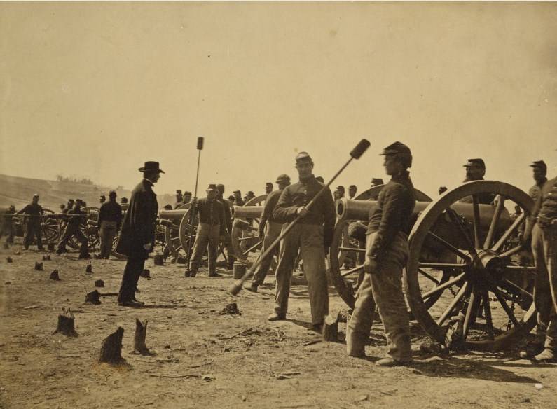
It's May 1, 1863. The bright and sunny sky in Chancellorsville, Virginia is interrupted sporadically by cannon fire. General's Robert E. Lee’s Army of Northern Virginia needs your help to stop an attempted flanking movement by General Joseph Hooker’s Army of the Potomac.

An artilleryman of New York’s First Artillery, lined up on the photo in front of his cannon, is wondering how he can maximize the chance to target the enemy by varying the cannon's inclination (angle). Artilleryman attempts some casual fires, that just disorients the opponent but do not reach the counterpart at all. As you guessed, the artilleryman tries to solve the problem analytically. As long as explosions rumble in the distance, he dips a feather from his pocket into an inkwell and writes the following equations.

First, the artilleryman supposes that the drag works directly against the velocity direction $v$. Due to the cannonball symmetry, the drag $D$ is in the opposite direction of $v$.

This means that the ratio of vertical and horizontal components of $v$ and $D$ should be the same

$$\frac{v_y}{v_x}=\frac{D_y}{D_x}.$$

At any following instant $t$, the horizontal and vertical forces acting on the cannonball ball are

$$F_x=D_x,\;\;\;F_y=-mg+D_y,$$

where $D_x$ is the horizontal and $D_y$ the vertical component of aerodynamic drag, and $gm$ is the gravity acceleration on the mass. Then, he obtains the drag components with the following equations

$$D_x=-\frac{\rho_aC_dA\left(v_x\sqrt{v_x^2+v_y^2}\right)}{2},\;\;\;D_y=-\frac{\rho_aC_dA\left(v_y\sqrt{v_x^2+v_y^2}\right)}{2},$$

where $\rho_a$ is the air density, $C_d$ is the drag coefficient and $A$ is the ball cross-sectional area. So, he describes the system' evolution with the following set of second order ordinary differential equations

$$\ddot{x}=-\frac{\rho_aC_dA\left(v_x\sqrt{v_x^2+v_y^2}\right)}{2m},\\ \ddot{y}=-g-\frac{\rho_aC_dA\left(v_y\sqrt{v_x^2+v_y^2}\right)}{2m}.$$

Finally, he starts to write the optimization problem. The cost function to minimize is represented by the vertical and horizontal velocity components $v^2$ that has to be minimized, and the constraints by the dynamics along with the boundary conditions at the initial and final point

$$\min \int_{t_i}^{t_f} v^2(\tau)d\tau\;\mathrm{s.t.}\;\Omega=\left\{ \dot{\mathbf{q}}=\begin{pmatrix}\dot{x}\\ \dot{v}\end{pmatrix}, \mathbf{q}_{t_i}=\begin{pmatrix}0\\0\\0\\0\end{pmatrix},\mathbf{q}_{t_f}=\begin{pmatrix}0\\ \alpha\\0\\0\end{pmatrix} \right\} $$

He tries to solve the equation with his knowledge from Optimal Control Theory but gives up soon. The variable space is too big. Confused about such lack in the feasibility of an analytic solution, the artilleryman tries a last attempt and searches for a solution on the web from his laptop. Suddenly, the artilleryman finds the following repository that could apply to his scenario

git clone https://bitbucket.org/adamseew/battle-chancellorsville.git

Exercise 1

The artilleryman soon understands how the code is structured. Classes are put in the src/ directory that contains the implementation while the include/ directory the definition. The sources wooden_ball.cpp and cannon_ball.cpp contain the dynamics. To perform the next step of the system we need to integrate the dynamics twice. integrator_rkn.cpp contains a modified version of RK4 integration algorithm. solver_shooting.cpp contains a non linear optimizer. Finally, the artilleryman learns that in order to start the algorithm he needs to perform following command

./run.sh

On the menu, he chooses the first voice. Let's help the artilleryman understand what's happening. What does the plot represent? What are the axis $x$ and $y$?

Exercise 2

Satisfied by your answer, the artilleryman runs again the algorithm and this time chooses the second voice. He is confused again. In the function program.cpp somebody forgot to implement the cannon_ball_example function. The function should perform the dynamics with different launching angle $\theta$ (the launches are performed by the run.sh script thus only one launch has to be implemented as in the previous example). $\theta$ will impact the velocity $v$ that is passed to the integrator as a state of the system. Use the implementation of wooden_ball_example as a hint and try to implement this example. Note that you will have two variables $(x,y)$, i.e., your vector that represents the initial boundary constraint $\mathbf{q}_{t_i}$ can be implemented

vectorn start_position(2);
start_position.set(0, 0.0);
start_position.set(1, 0.0);

Exercise 3

Face towards the direction of the sky, the artilleryman yells "thank you brave man from the future"! But not everything is done. With the previous example, we have performed just a set of random launches. Let's execute the algorithm again choosing the third voice. This time the enemy, at $x_{t_f}= (605, 0)^T$ meters is targeted. As the artilleryman will learn soon, the optimal solution is not always achievable. In the great majority of cases, the optimum can be reached only within a specific tolerance.Try to perform the two different tolerance indexes and note the difference.

The artilleryman is finally ready to reach his target when suddenly he learns that somebody forgot to save the initial velocity output from the optimizer. Let's help the artilleryman one more time and save the output in a file called initial_v.dat!